Showing posts with label 2. Power BI / SSBI. Show all posts

Wednesday, March 25, 2026

Solving Power BI Drillthrough Limitations for Multi-Period Daily Analysis

                                                                                                                          Check list of all posts


Background

In many Power BI reports, the main page is filtered at a period level—for example, a selected month such as February 2025.

When users drill through to a detail page, the requirement often expands to:

  • display all daily records for the selected period, and
  • at the same time display all daily records for a comparison period

The comparison period can be:

  • previous month
  • next month
  • prior year
  • previous quarter
  • or any custom offset

The Core Challenge

The drillthrough page receives a filter from DimDate, which defines the selected period.

This creates a fundamental limitation:

  • visuals using DimDate only show the selected period
  • another period cannot be shown simultaneously using the same relationship

👉 A single connected date dimension can only propagate one active filter context.


Initial Approach: Connected DimDate (RolePlay)

A common first attempt is:

  • create a second date table: DimDate (RolePlay)
  • connect it to the fact table
  • use it for the comparison period

Design

  • DimDate → drives drillthrough (selected period)
  • DimDate (RolePlay) → drives comparison period

Why This Approach Fails (Performance)

Connecting DimDate (RolePlay) directly to the fact table introduces significant performance overhead.

  • More complex filter propagation
    Multiple date relationships force the engine to evaluate more complex filter paths, reducing optimization efficiency.
  • Increased formula engine workload
    The engine spends more time resolving competing date contexts instead of pushing simple queries to the storage engine.
  • Reduced cache reuse
    Additional date paths create more unique filter combinations, which limits cache effectiveness.
  • Slower queries at scale
    For large models with daily granularity and complex measures like [MeasureX], this results in noticeably slower report performance.

👉 In short, multiple connected date tables increase computation cost and reduce performance efficiency.


Final Solution: Disconnected DimDate (RolePlay) + TREATAS

A better design is:

  • keep only one connected DimDate
  • convert DimDate (RolePlay) into a disconnected helper table
  • use TREATAS inside measures to control the date context

Key Idea

👉 Do not rely on relationships — control date context explicitly in the measure.


Implementation Pattern

1. Connected date table

  • DimDate remains the only table connected to the fact table
  • handles drillthrough and standard filtering

2. Disconnected helper table

  • DimDate (RolePlay) has no relationship
  • used only to generate comparison-period rows

3. Measure logic

Comparison Period MeasureX =
VAR _RolePlayDate =
SELECTEDVALUE('DimDate (RolePlay)'[Date])
RETURN
CALCULATE(
[MeasureX],
REMOVEFILTERS('DimDate'), -- remove drillthrough filter
TREATAS({_RolePlayDate}, 'DimDate'[Date]) -- apply desired date
)

How It Works

Step 1 — Remove original filter

  • clears the drillthrough period (e.g., February)

Step 2 — Apply new date

  • injects comparison period date (e.g., January)

Result

  • no conflicting filters
  • precise control of date context
  • correct results for both periods

Benefits

  • Better performance → simpler filter paths
  • Cleaner model → single source of truth
  • More flexible → supports any time offset
  • Easier to maintain → explicit logic

Recommended Pattern

  • ✅ One connected DimDate
  • ✅ One disconnected DimDate (RolePlay)
  • ✅ Use TREATAS in [MeasureX]
  • ❌ Avoid multiple connected date tables

Conclusion

The limitation comes from the fact that a connected date dimension can only support one active period at a time.

Instead of introducing additional connected date tables, the optimal solution is:

  • use a disconnected helper table
  • explicitly override date context using TREATAS

Executive Summary

Use a single connected DimDate, a disconnected helper date table, and override date context in [MeasureX] using REMOVEFILTERS and TREATAS. This avoids performance issues and enables flexible multi-period analysis in drillthrough pages.


Monday, December 8, 2025

Avoiding the Performance Trap: Files-Based Incremental Loading for Large Folder Power Query Sources

 Executive Summary

Organizations increasingly rely on Power BI to analyze data stored in shared folders containing hundreds or even thousands of flat files produced by modern Big Data platforms. While this file-based architecture supports strong data management practices—such as lineage, auditability, and replayability—it creates a major refresh performance challenge: Power BI tries to read every file during every refresh unless incremental refresh is implemented correctly.

This blog provides:

  • A complete, practical blueprint for files-based incremental loading

  • Clear explanations of the three types of refresh behaviors

  • Deep insight into why performance issues occur

  • A comprehensive list of common pitfalls, with reasons and consequences

When implemented properly, incremental refresh transforms a slow, hour-long refresh into a fast, stable, 5–10 minute refresh—even with years of historical files.


1. Why Do Big Data Platforms Produce So Many Files? 

Modern data platforms are designed around append-only ingestion. Instead of updating existing data, they continuously write small, time-stamped files—daily, hourly, or by batch. This pattern:

  • Ensures auditability

  • Preserves full historical lineage

  • Allows efficient reprocessing and rollback

  • Aligns with cloud data lake best practices

The result is inevitable: massive file counts in shared locations accessed by Power BI.

To make Power BI perform well against such sources, incremental loading is essential.


2. What Is Files-Based Incremental Loading?

Databases support incremental refresh naturally because they include date columns and optimized partition indexes. Flat files do not.
To mimic database-like behavior for folder sources, Power BI must:

  1. Extract a date value from each file name (FileDateTime).

  2. Use RangeStart and RangeEnd parameters to select only the relevant files.

  3. Apply incremental refresh policies that freeze historical data and refresh only recent partitions.

This reduces unnecessary work and provides consistent, efficient refresh cycles.


3. High-Level Architecture

The architecture follows a clean, layered design:

  1. Folder Source: Power BI connects to a shared folder containing many files.

  2. Staging Layer: Extracts a date value from each file name, then filters files using RangeStart and RangeEnd—before expanding file contents.

  3. Fact Layer: Expands and transforms only the filtered files.

  4. Incremental Refresh Engine: Power BI Service partitions and manages historical vs. incremental data.

This separation ensures Power BI reads only what is needed.


4. Core Implementation Pattern 

4.1 Create RangeStart and RangeEnd parameters

These DateTime parameters define the boundaries of the incremental refresh window. Desktop uses them literally; the Service replaces them dynamically.

4.2 Derive FileDateTime from the file name

For example, if a file name begins with a date such as “20230102,” interpret it as January 2, 2023. This becomes the date used for filtering and partitioning.

4.3 Filter early, before expanding file contents

Filter the list of files so only those whose FileDateTime is within the desired window are expanded and processed.
The correct pattern is:

  • FileDateTime greater than or equal to RangeStart

  • FileDateTime strictly less than RangeEnd

4.4 Apply incremental refresh

Define how many years of history to keep and how many days/weeks/months to refresh.
Power BI then creates partitions and ensures only recent partitions are refreshed going forward.


5. Understanding the Three Refresh Scenarios

Power BI handles refreshes differently in Desktop and in the Service. Misunderstanding these differences often leads to wrong expectations or incorrect troubleshooting.


Scenario 1 — Power BI Desktop: Development Mode

What actually happens

Desktop loads exactly the files that fall between the RangeStart and RangeEnd parameters you define.
It does not create partitions.
It does not perform dynamic date substitution.
It does not optimize file scanning.

Reason

Desktop is built for development and debugging—not for processing large historical datasets.

What to expect

  • Small date window → fast and smooth

  • Large date window → very slow, memory-heavy, or crashes

Result if misused

Developers mistakenly think incremental refresh “doesn’t work” because Desktop behaves like a full refresh when too many files are included.

Best practice

Use only a small date testing window (1–3 days).


Scenario 2 — Power BI Service: Initial Full Load (First Refresh After Publishing)

What actually happens

Power BI Service completely ignores the Desktop parameter values and instead loads:

  • The entire historical dataset required by your incremental refresh policy

  • All partitions needed for historical storage

This is the only time Power BI performs a complete historical load.

Reason

Power BI must build the entire partition structure for incremental refresh to work.

What to expect

  • This refresh may take a long time, depending on data volume.

  • It prepares the model for efficient future incremental refresh cycles.

Result if misunderstood

Teams think incremental refresh is “slow,” not realizing this is a required setup step.
Multiple republishing resets the partition structure and forces another full load.

Best practice

Allow the first refresh to complete and avoid unnecessary republishing.


Scenario 3 — Power BI Service: Ongoing Incremental Refresh (Normal Operation)

What actually happens

After partitions are built:

  • Only recent partitions (for example, the last 7 days) are refreshed

  • Older partitions remain frozen

  • Only new files are processed

Reason

Incremental refresh is designed to process only new data (“delta” refresh).

What to expect

  • Large performance improvement

  • Stable refresh durations

  • Minimal system load

Result if implemented incorrectly

If filtering is incorrect, file structures are bad, or partitions are too granular, Power BI may still scan all files or reprocess excessive partitions.

Best practice

Optimize filtering, folder structure, and partition granularity to maximize efficiency.


6. Benefits of Files-Based Incremental Loading

  • Massively reduced refresh time

  • Stable, predictable refresh performance

  • Historical data becomes immutable and reliable

  • Reduced workload on gateways and file systems

  • More efficient troubleshooting and data governance


7. Common Pitfalls & How to Avoid Them

Pitfall 1 — Incorrect Filter Pattern (Not Left-Inclusive, Right-Exclusive)

Reason

If the filter allows FileDateTime values on both boundaries, partitions overlap.

Result

  • Duplicate rows

  • Incorrect totals

  • Reprocessed files

  • Wrong business results

Fix

Always include the lower boundary and exclude the upper boundary.


Pitfall 2 — Too Many Partitions (Daily/Weekly/Monthly)

Reason

Power BI creates one partition per time unit.
If you define sixty daily partitions, Power BI scans the entire folder sixty times.

Result

  • Extremely long refresh

  • Heavy load on gateway and file server

  • Incremental refresh becomes slower than full refresh

Fix

Use weekly or monthly partitions for large file volumes, and keep the refresh window short.


Pitfall 3 — Keeping All Files in One Large Flat Folder

Reason

File systems do not support partition-aware scanning.
Power BI must enumerate every file repeatedly across partitions.

Result

  • Very slow metadata scanning

  • Refresh performance degrades as the folder grows

  • Service load increases exponentially

  • Incremental refresh loses effectiveness

Fix

Organize files into year/month subfolders so Power BI can skip entire folders.


Pitfall 4 — Filtering Files Too Late in the Query

Reason

If filtering is applied after expanding file contents, Power BI must load every file before deciding which ones to discard.

Result

  • Essentially becomes a full refresh

  • Very slow processing

  • High memory usage

Fix

Apply FileDateTime filtering immediately after reading folder metadata.


Pitfall 5 — Large Parameter Window in Desktop

Reason

Desktop uses the parameter values literally and loads all files in the range.

Result

  • Desktop freezes or crashes

  • Development slows dramatically

Fix

Keep Desktop ranges small (1–3 days).


8. Summary

Folder-based incremental refresh is powerful—but delicate.
When implemented correctly, it resolves one of the biggest performance barriers in Power BI: efficiently handling very large collections of flat files.

Success depends on:

  • Using the correct filtering logic

  • Managing partition granularity

  • Designing a smart folder structure

  • Filtering early

  • Using small development windows

  • Understanding Desktop vs. Service refresh behavior

With these principles, even large multi-year file archives refresh efficiently, reliably, and predictably.


----------------------------------------------------
Journal

March 1: dataset refresh not failed, and data from Feb 27 not ready.

Refresh window = March 2026;  Drop partition 2026-03; Re-query source for: WHERE Date >= 2026-03-01 AND Date < 2026-04-01; 


Step C — Keep Historical Partitions Frozen

These are NOT touched:

2025-01 → 2026-02

Friday, December 5, 2025

Avoid Reusing Large Folder-Based Power Query Sources — Clarifying a Common Misunderstanding

 Executive Summary

Power BI makes it easy to ingest data from folders containing many files, but when the volume reaches thousands of files and multiple gigabytes, refresh performance becomes a serious concern. A common misunderstanding is assuming that when multiple Power Query objects reference the same base folder query, Power BI automatically “reuses” that data. Unfortunately, this is not how the Power BI refresh engine works.

When downstream queries depend on a Power Query folder source—and all are enabled for load—Power BI evaluates each query independently. This means the folder is scanned multiple times during refresh, even though the queries appear to share the same base logic. The impact can be dramatic: refreshes become slow, unstable, and unnecessarily heavy on the underlying storage system.

This document explains why this happens, what the risks are, and how to redesign the dataset so the folder is loaded once, while all other logic is rebuilt efficiently inside the model using DAX calculated tables. This approach eliminates redundant IO, improves refresh performance, and clarifies a widely misunderstood aspect of Power Query behavior.


Requirements

The dataset contains three Power Query components:

  1. Query 1

    • Reads from a folder containing ~2000 files totaling ~4 GB.

    • Represents the detailed transactional dataset.

  2. Query 2

    • Referenced from Query 1, applying additional transformations.

  3. Query 3

    • Also referenced from Query 1, extracting a different view of the same data.

All three queries are currently enabled for load into Power BI.

The main requirement is:

Refresh the dataset efficiently and ensure the large folder is not scanned multiple times.


Analysis

Although Queries 2 and 3 are visually created by referencing Query 1 within Power Query, this does not imply reuse or caching during refresh. Power BI treats every loaded query as an independent evaluation path.

Behind the scenes:

  • Each loaded query is evaluated separately

  • Each query’s full dependency chain is executed

  • Folder connectors do not share cached results

This means:

  • Query 1 triggers a full folder scan

  • Query 2 triggers another full folder scan

  • Query 3 triggers yet another full folder scan

Total effect:

  • Three full scans of ~2000 files

  • Three ingestion cycles of ~4 GB each

  • ~12 GB of IO per refresh instead of 4 GB

This leads to:

  • Slow refresh duration

  • Higher chance of refresh timeout

  • Increased load on upstream storage

  • Poor scalability as logic grows

This is a common misunderstanding: referencing a query in Power Query does not guarantee shared evaluation.


Solution

To eliminate redundant folder scans, the dataset should be redesigned so that:

✔ Only one Power Query object loads the large folder

This ensures the folder is scanned once.

✔ Downstream logic is removed from Power Query

Queries derived from the folder source should not be loaded, preventing multiple evaluations.

✔ All additional “views” are rebuilt inside the model using DAX calculated tables

These tables mimic the original Power Query outputs but are computed in-memory, without touching the folder source again.

This design achieves:

  • A single ingestion point

  • Faster refresh performance

  • Reduced infrastructure load

  • A cleaner, more maintainable model


Implementation

1. Keep Query 1 as the only loaded Power Query object

Query 1 remains the sole location where the folder is read:

  • Query 1 → Enable Load = On

This becomes the single ingestion pipeline for the dataset.


2. Disable load for Query 2 and Query 3

These downstream queries should not trigger additional refresh paths.

In Power Query:

  • Right-click Query 2 → uncheck Enable Load

  • Right-click Query 3 → uncheck Enable Load

They remain as reference definitions, but no longer evaluate during refresh.


3. Rebuild the logic of Query 2 and Query 3 using DAX calculated tables

After Query 1 loads into the model, replicate the logic of the outdated Power Query transformations using DAX calculated tables.

This includes:

  • Summaries

  • Filters

  • “Latest record” logic

  • Grouping or aggregation

  • Business-specific views

These DAX tables are:

  • Computed once after refresh

  • Built from the in-memory data of Query 1

  • Functionally identical to the old Power Query outputs

  • Much faster and more reliable

  • Not dependent on folder scans

Once created, they replace the old Query 2 and Query 3 in the model.


4. Remap the data model and reports

With the new DAX tables in place:

  • Update relationships to point to the new calculated tables

  • Adjust measures and calculated columns if needed

  • Update report visuals to reference the new tables

  • Remove Query 2 and Query 3 from the model after migration is complete

From the user’s perspective, all visuals and logic behave exactly the same.

From the engine’s perspective, refresh is now far more efficient.


5. Validate the refresh and reporting behavior

After implementation:

  • Refresh the dataset

  • Confirm that refresh time is significantly reduced

  • Verify that the folder is scanned only once

  • Ensure all reports continue to function correctly

  • Finalize model cleanup

This completes the migration from a multi-scan design to a single-scan, optimized architecture.


Conclusion

A major misunderstanding in Power BI development is assuming that referencing a Power Query object automatically reuses previously loaded data. When dealing with large folder-based sources, this misunderstanding can lead to multiple unnecessary full-folder scans and severe performance degradation.

The correct architectural approach is:

  • Load the folder once

  • Disable downstream Power Query loads

  • Rebuild the additional views as DAX calculated tables

  • Remap the model and reports accordingly

This ensures a scalable, efficient, and maintainable dataset that refreshes quickly and avoids redundant IO.

Wednesday, February 12, 2025

Simplifying Power BI Architecture: A Consulting Experience

                                                                                                                      Check list of all posts

When working on Power BI projects, one of the most common challenges involves optimizing the architecture for stability, performance, and simplicity. I recently had the opportunity to consult on a Power BI implementation that faced significant issues, and this article details the steps taken to simplify the architecture and resolve the core problems.

Existing Problems

The original implementation had several critical issues:

  1. Report Stability Issues

    • When many users accessed the report simultaneously, the system would crash or time out, leading to significant frustration.

  2. Poor Performance

    • Reports took between 1.5 to 3 minutes to load, regardless of the data volume. To address this, users had to rely on "Buttons -> ‘Apply all slicers’," which added complexity and did not address the root cause.

  3. Overly Complex Architecture

    • The architecture utilized mixed modes, including DirectQuery with complex parameter passing, dataflows for pre-populating aggregate-level data, and materialized views to improve SQL performance. This led to a convoluted system that was difficult to manage and optimize.


Existing Architecture

The architecture relied on three main components:

  1. DirectQuery Mode

    • This mode was used extensively, with complex parameter passing from the interface, but it caused system instability and performance bottlenecks.

  2. Dataflows

    • These were used to pre-populate aggregate-level data, adding another layer of complexity and maintenance.

  3. Materialized Views

    • SQL materialized views were implemented to speed up query performance but introduced a significant maintenance overhead, including a one-year refresh schedule.


Simplifying the Architecture

To address these issues, I implemented a three-step plan to simplify the architecture:

Step 1: Eliminate DirectQuery

The first step was to remove DirectQuery by deeply understanding the business requirements and compressing the data as much as possible. This step involved:

  • Requirement Analysis:

    • Understanding what data and level of granularity were truly necessary.

  • Data Compression:

    • Reducing data volume through effective summarization and removal of unnecessary fields.

  • Optimized DAX Queries:

    • Refactoring DAX formulas to improve efficiency.

Outcome:

  • Resolved system availability issues, allowing multiple users to access reports simultaneously without crashes.

  • Decoupled the reports from the database, enabling data retrieval from the cloud and improving stability.

Step 2: Remove Dataflows

The next step was to eliminate dataflows and bring all necessary data directly into Power Query. This was achieved by:

  • SQL Performance Tuning:

    • Enhancing SQL query performance to fetch data efficiently without relying on intermediate dataflows.

  • Direct Integration:

    • Using Power Query to load and transform data directly, simplifying the overall data pipeline.

Outcome:

  • Reduced maintenance time and complexity.

  • Improved data loading speeds significantly.

Step 3: Replace Materialized Views

Finally, we eliminated the dependency on materialized views by querying the database directly from Power Query. This involved:

  • SQL Query Optimization:

    • Leveraging similar performance tuning techniques as in Step 2 to improve query execution times.

  • Real-Time Data Access:

    • Enabling Power Query to retrieve data as needed, removing the need for pre-populated materialized views.

Outcome:

  • Eliminated the one-year materialized view refresh schedule.

  • Simplified the system by removing an additional layer of abstraction.


Final Results

From the User Perspective:

  • System Availability: Reports are now available 24/7, even with multiple users accessing them simultaneously.

  • Improved Performance: The slowest report load time is reduced to about 10 seconds, even with maximum data volume.

From the Technical Perspective:

  • Eliminated Maintenance Overheads:

    • Removed the one-year refresh time for materialized views.

    • Eliminated the one-hour dataflow refresh time.

  • Simplified Architecture:

    • Reduced complexity by eliminating DirectQuery, dataflows, and materialized views.

  • Flexible Refreshing:

    • The system can now be refreshed anytime as needed without additional overhead.


Conclusion

By addressing the root causes of instability and poor performance, and by simplifying the Power BI architecture, the system became more reliable, faster, and easier to manage. This consulting experience highlights the importance of deeply understanding requirements, optimizing SQL performance, and leveraging Power Query to build a streamlined, high-performing Power BI solution.

Friday, July 26, 2024

Unlock the Full Potential of Power BI with Row-Level Security (RLS)

                                                                                                                         Check list of all posts

Objective

Using a single table to control all static and dynamic Row-Level Security (RLS) in Power BI has several advantages:

Centralized control: With a single table, you can centralize all your RLS rules and permissions in one place, which can make it easier to manage and maintain your data model. This can be particularly useful if you have a large number of users, groups, and data sets that need to be managed.

Improved efficiency: A single table can help to streamline the process of managing RLS permissions, as you only need to update a single table to make changes to the permissions. This can save time and reduce the risk of errors, particularly if you have a large number of rules or permissions to manage.

Simplified troubleshooting: With all your RLS rules and permissions in a single table, it can be easier to troubleshoot any issues or problems that may arise. You can use the table to quickly identify and fix any errors or inconsistencies in your RLS rules, which can help to ensure that your data model is accurate and up-to-date.

Overall, using a single table to control all static and dynamic RLS in Power BI can help to improve the efficiency, simplicity, and accuracy of your data model, and make it easier to manage and maintain your RLS rules and permissions.

We want to enhance our use of Power BI by consolidating all our Row-Level Security (RLS) requirements into a single role. Currently, we have to define static RLS and dynamic RLS separately, and we have to set up multiple roles for specific dimensions in static RLS. Additionally, we have different areas for each static RLS. To address this, we aim to combine all data into a single dataset and create a single role for all RLS to achieve the following goals:

1) Combine static and dynamic RLS, allowing users to access only their own data and the data they are allowed to see based on their role or group membership.

2) Create a static RLS for multiple dimensions, such as product and customer dimensions.

3) Create a single role for each dimension, such as multiple products.

This document will provide a solution that guides you through the process, from the database to the final reports.

Sample data setup (SQL server)
DROP TABLE IF EXISTS dbo.CYFact;
Go
CREATE TABLE dbo.CYFact(
UserID varchar(10) ,
Product varchar(10) ,
Customer varchar(10) ,
Sales varchar(10) 
)
Go
insert into dbo.CYFact values 
('U1','P1','C1',1),
('U1','P1','C2',2),
('U1','P2','C1',3),
('U1','P2','C2',4),
('U2','P1','C1',5),
('U2','P1','C2',6),
('U2','P2','C1',7),
('U2','P2','C2',8)
Go
DROP TABLE IF EXISTS dbo.CYRLS;
Go
CREATE TABLE dbo.CYRLS(
ID varchar(10) ,
Email varchar(100) ,
IsDynamicRLS varchar(10),
ProductStaticRLS varchar(10) ,
CustomerStaticRLS varchar(10) 
)
Go
insert into dbo.CYRLS values 
('U1','U1@Test.com','Yes','P1','C1'),
('U1','U1@Test.com','Yes','P2','C1'),
('U2','U2@Test.com','No','None','C1')
Go
DROP TABLE IF EXISTS dbo.CYUser;
Go
CREATE TABLE dbo.CYUser(
ID varchar(10),
Email varchar(100) ,
)
Go
insert into dbo.CYUser values 
('U1','U1@Test.com'),
('U2','U2@Test.com')

Go
DROP TABLE IF EXISTS dbo.CYProduct;
Go
CREATE TABLE dbo.CYProduct(
ID varchar(10))
Go
insert into dbo.CYProduct values 
('P1'),
('P2')
Go
DROP TABLE IF EXISTS dbo.CYCustomer;
Go
CREATE TABLE dbo.CYCustomer(
ID varchar(10))
Go
insert into dbo.CYCustomer values 
('C1'),
('C2')

Data Model
Assuming that there are only one fact and three dimensions with a typical star schema. Please note the RLS is a disconnected table with all dimensions and fact tables.


Security Logic
We use 3 sample records below to demonstrate all cases we try to achieve.

  • U1 supports dynamic RLS, meaning that U1 can only access his data to the Fact sales table.
  • U1 supports static RLS for the product dimension, with two products P1 and P2
  • U1 supports static RLS for the customer dimension, with one customer C1 only
  • U2 doesn't support dynamic RLS, meaning that U2 can access all data. For example, he can access U1 data.
  • U2 doesn't support static RLS for the product dimension, meaning that U2 can access all products.
  • U2 supports static RLS for the customer dimension, with one customer C1 only.
Role implementation

CYUser

VAR _DimRLS =
    CALCULATETABLE (
        VALUES ( 'CYRLS'[IsDynamicRLS] ),
        'CYRLS'[Email] = USERPRINCIPALNAME ()
    )
VAR _RLS =
    SWITCH (
        TRUE (),
        _DimRLS = "No", TRUE (),
        [Email] = USERPRINCIPALNAME (), TRUE (),
        FALSE ()
    )
RETURN
    _RLS

CYProduct

VAR _DimRLS =
    CONCATENATEX (
        CALCULATETABLE (
            VALUES ( 'CYRLS'[ProductStaticRLS] ),
            'CYRLS'[Email] = USERPRINCIPALNAME ()
        ),
        'CYRLS'[ProductStaticRLS]
    )
VAR _RLS =
    SWITCH (
        TRUE (),
        CONTAINSSTRING ( _DimRLS, "None" ), TRUE (),
        CONTAINSSTRING ( _DimRLS, [ID] ), TRUE (),
        FALSE ()
    )
RETURN
    _RLS

CYCustomer

VAR _DimRLS =
    CONCATENATEX (
        CALCULATETABLE (
            VALUES ( 'CYRLS'[CustomerStaticRLS] ),
            'CYRLS'[Email] = USERPRINCIPALNAME ()
        ),
        'CYRLS'[CustomerStaticRLS]
    )
VAR _RLS =
    SWITCH (
        TRUE (),
        CONTAINSSTRING ( _DimRLS, "None" ), TRUE (),
        CONTAINSSTRING ( _DimRLS, [ID] ), TRUE (),
        FALSE ()
    )
RETURN
    _RLS

Test result

No Security ( Admin )


U1: User 1 login


U2: User 2 login


Note 1: If a user is assigned to two roles for row-level security (RLS) in Power BI, they will have access to the data that is allowed by the rules associated with both of those roles. This means that the user will be able to see all of the data that is allowed by the rules for either of the two roles. However, we try to assign everyone to a single role, driven by the table defined.

Note 2:  If a user has no role assigned with row-level security (RLS) in Power BI, they will not be able to access the data in the dataset. This is because RLS is designed to restrict access to data based on the user's role, and a user who has no role will not have any access to the data.

Note 3: To give people full access to data in Power BI using row-level security (RLS), you can create a role with no rules, or you can create a rule that allows access to all rows of data.
To create a role with no rules, you can simply define the role in the Power BI service and assign users to it. This will allow those users to see all of the data in the dataset, regardless of any other roles they may be assigned to.
Another way to do it is to assign this user to the contributor for the workspace where the dataset resides.

Note 4 The key to understanding RLS is that we implement RLS on the Power dataset. So, first of all, we need to figure out the fundamental permissions to Power BI datasets, which is the write permission. If a user has written permission on a Power BI dataset, then RLS won’t apply for this user. Why? Because the user can edit permission for these roles. If the user doesn’t have permission to write the dataset, RLS is fully enforced, no matter where the user has access to this dataset, in the original workspace, or any apps and shared links.
 Who has write permission for a dataset?
The user has access to the same workspace of the Power BI dataset and has permission as
• Admin
• Member
• Contributor
Who has no write permission on the dataset?
There are three cases where people have no write permission:
1) Report is in the same workspace as dataset. The user has permission as Viewer only.
2) Report is in a different workspace than the dataset. Users can be assigned to any security group, however these users should have only read, or build permission to the dataset.
3) Reports are accessed by a shared links
4) Reports are accessed by an apps
The diagram below illustrates all cases below.


Note 5: The "apply security filters to both directions" option in Power BI Row-Level Security (RLS) is used to enforce security filters in both the filters and visuals panes of a report. This can be useful for ensuring that users only see data that they are authorized to see, regardless of how they interact with the report.
For example, consider a report that contains a visual showing sales data for different products and customers. You have set up RLS rules to limit access to certain products based on the user's role, but you want to ensure that users cannot see data for customers that they are not authorized to see, even if they try to manipulate the filters or visuals to see data for other customers. In this case, you could use the "apply security filters to both directions" option to enforce the security filters in both the filters and visuals panes of the report.  However, this solution might not be the best, as there are two problems: 1) when the transaction table is huge, then it will result in poor performance; 2)  You might want customers, even if you don't have sales with the context of filters.

Note 6: User group to setup permissions:
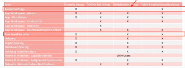


Note 7:  Why LOOKUPVALUE method is much more flexible than  USEPRINCIPALNAME: 
Dynamic security is a feature that allows you to change the level of access that users have to data in a Power BI report or dashboard at runtime. It allows you to specify which data a user can see based on their identity or role within an organization.
One way to implement dynamic security in Power BI is by using the LOOKUPVALUE function in combination with a security table. The security table is a table in your Power BI dataset that defines the level of access that different users or groups have to different data.
The LOOKUPVALUE function allows you to look up a value in a table based on a matching condition. In the context of dynamic security, you can use the LOOKUPVALUE function to look up the level of access that a user has to a particular data element in the security table, based on their user name or group membership.
For example, suppose you have a Power BI report that displays sales data for different products and customers. You can use the LOOKUPVALUE function to check the security table to see if the current user has access to the data for a particular product or customer. If the user has access, the LOOKUPVALUE function will return the value "Allow" and the user will be able to see the data. If the user does not have access, the LOOKUPVALUE function will return the value "Deny" and the user will not be able to see the data.
Using the LOOKUPVALUE function and a security table allows you to implement dynamic security in a flexible and scalable way. It allows you to control access to data at a granular level and to change the level of access that users have to data on the fly, without the need to update the report or dashboard.
By contrast, the USEPRINCIPALNAME function allows you to filter data based on the current user's login name. While this can be useful in some cases, it is less flexible than using a security table and the LOOKUPVALUE function, as it does not allow you to specify different levels of access or to easily change the level of access that users have to data.


Note 8:   Sample Implementation case of Row-Level Security (RLS)

Current Setup and Objective

Given that we have three different layers for Power BI implementation:

1. App Layer – Analytics

2. Dashboards/Reports Layer - SECURE_PROD

3. Semantic Model Layer - SECURE_Data

The Model is shared and located in a separate workspace (SECURE_Data). Dashboards/Reports are in a separate workspace (SECURE_PROD), where the shared Model is used. All dashboards/reports are organized in Power BI apps.

Ensure that when a specific employee logs in, they can only view their assignments for planned and actual data, while all other dashboards should not be impacted.

 Analysis

Implementing RLS can effectively resolve this visibility issue. The challenge lies in deciding whether to utilize a consolidated or separate model.

Separated Model Strategy

Advantages:

- Ease of Implementation: Implementing RLS on a separate model does not impact the central Model.

- Standardized Process: The implementation process is standardized, making it straightforward.

- Maintenance Simplicity: The separate model is easier to maintain due to its independence.

Disadvantages:

- Dual Maintenance Required: Any changes requiring updates in both models increase maintenance effort.

- Complex Separation: Defining a clear boundary between models is challenging due to many involved parameters.

- Dashboard Transition: Employees need to switch to the new model, potentially necessitating adjustments to the overview pages, which could become a considerable risk to implement.

Consolidated Model Strategy

Adding security to the data model will impact all dashboards, which is not desirable. The solution is to somehow enhance the current model by leveraging an “Inactive Relationship” for RLS, which should affect only dashboards that need to have RLS, and leave other dashboards unchanged.


Advantages:

- Single Model Management: Maintains a single model, avoiding duplicated efforts and simplifying management.

- Seamless Integration: All existing parameters and functions remain effective without needing alterations.

- Unified Dashboard Access: The employee dashboard points to the same model, ensuring consistency.

Disadvantages:

- Dashboard Adjustments Needed: Modifications to dashboard measures are required to activate the RLS features.

Implementation Details

1. The model includes an inactive relationship, which is currently used only for presentation purposes and is not operational in any DAX formulas. Also, `NetworkLoginName` is used for consistency.

2. The role  for a specific AD group has been configured for data viewing permissions.

3. DAX solutions have been implemented. Note that the functions `USERELATIONSHIP` and `CROSSFILTER` are not yielding the expected results.


MeasureX (RLS) =
VAR Email =
    
SELECTEDVALUE ( Users[Email] )
RETURN
    
IF (
        
ISBLANK ( Email ),
        [MeasureX],
        
CALCULATE (
            [MeasureX],
            'DimensionX'[Email] = 
Email
        
)
    
)


Deployment Details - Adding a Person or Group to RLS

 To add a person or a group to the RLS, you need to add this security to four different places:

On the Power BI app side ( at the audience level) .

On the dashboard/report side ( at the report level, not the workspace level, as you don't want people to access the report workspace)

On the semantic model ( at the model level, not the workspace level, as you don't want people to access the report workspace)

On the RLS security setting.

If a user has access to the dataset with Build, Share, or Reshare permissions but does not have Write access, you also need to add the user to the Security settings for the semantic model. However, if the user has Write access to the dataset, then it is not necessary to add them to the Security settings for the semantic model. Typically, we apply the first case.